This Case Study investigates how we carried out a survey of a local golf course, using a combination of different data types and sources. Whilst this is not intended to be a definitive solution we will introduce some useful tools that can you may use elsewhere.
The purpose of the survey was to identify highs and lows for drainage and to determine surface areas of fairways, greens and tee boxes so that surface treatments can be accurately applied, including chemical sprays. As an extra exercise, the slopes on greens were mapped.
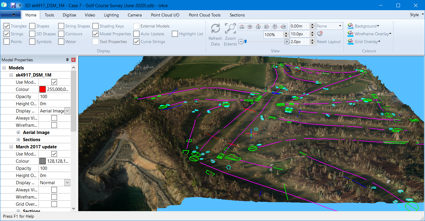
3D view of Longcliffe Golf Course Survey
The survey project is ongoing and as with any golf course changes are constantly being made and the course updated. Many of the bunkers were reshaped and refilled to give them both consistency and visual impact and some tee boxes replaced. The driving range is being revamped, which is the topic of another Case Study.
Fairways are tree-lined, so traditional total station surveys were not appropriate, so we relied on GNSS. But in the early stages, signal strength and tree shadowing caused problems. At one stage we stood in the middle of the 18th fairway, clear of any trees for over 30mins unable to get a signal. Thankfully, matters later improved!

GNSS Survey
The first GNSS survey was carried out in 2009 which included surveying the fairway centre lines and identifying the highest and lowest points on the course for drainage purposes.
The course elevation changes from 132m at its highest to 75m at its lowest; a total height change of 57m. The tee to green centreline of each hole was surveyed, also identifying elevation changes.
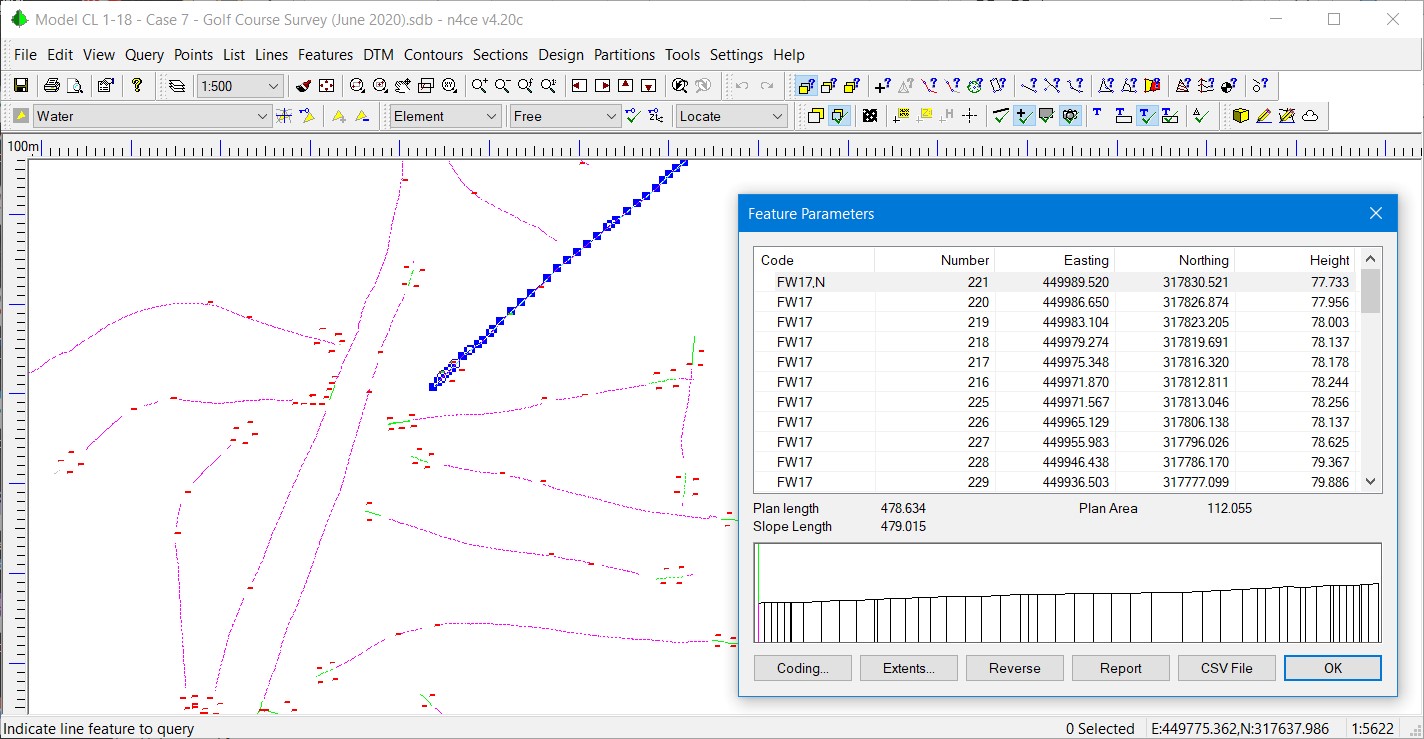
Tee to Green Centrelines
The greens, bunkers and ditches were surveyed together with other obstacles, like bunds. The sprinkler heads around each green were identified so that we could come back later and carry out a total station survey of each green for slopes - but see later.
Since it wasn’t practical to do a full survey of tree and fairway outlines, we looked at other appropriate data sources. Whilst it’s possible to get imagery from Google Maps, these are neither georeferenced nor orthorectified. But there are sources that provide this information.
Our photography was sourced from GetMapping but other sites are available, like Emapsite. But be careful, as there may be images flown at different times. Early images are cheaper but maybe missing detail.
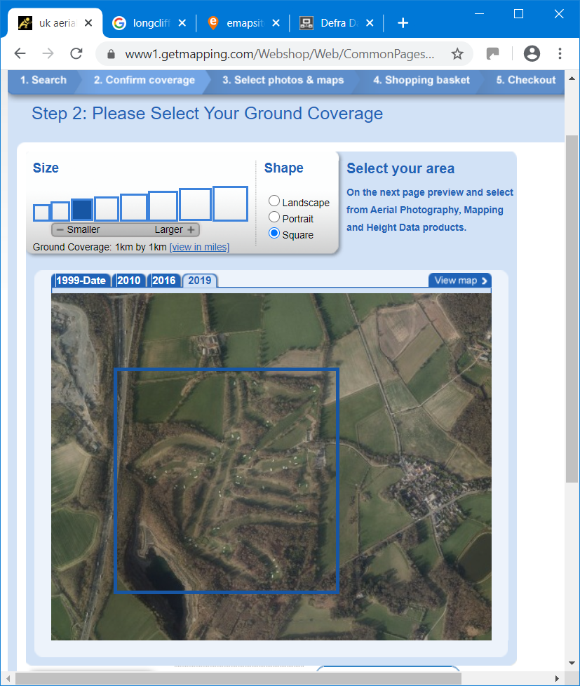
GetMapping - Selecting the Coverage and Flown Date
Our first image was dated 2006 – 2013 but was missing detail that had changed. We subsequently updated the imagery and we’re using the latest one here, dated 2019 and costing £77+vat. You can also purchase LiDAR grided data from these sites, but we used data freely available from the Environment Agency.

1km Square Georeferenced and Orthorectified Image of Longcliffe Golf Course
From this photography, the tree canopy can be identified, along with the fairway outline. These can be digitised in n4ce providing useful information for the green staff but in 2D.
Since our ground survey was restrictive and didn’t provide levels everywhere, we filled out using LiDAR data from the Environment Agency. This is freely available from their website, but you will need to know which OS cells you are interested in, as your site might fall across a number of cells. In our case, the site fell within SK41NE.
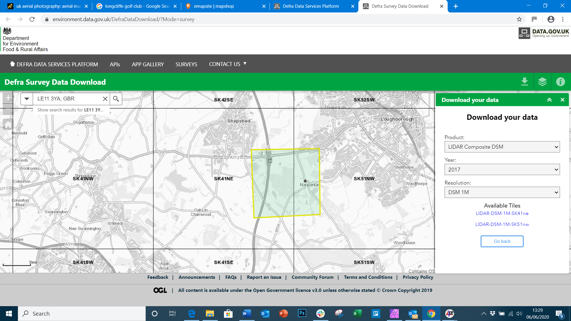
Environment.data.gov.uk
The latest data was flow in 2017 and updated in 2018, with various data formats available. We selected 1m grid intervals and download both DSM and DTM. The DTM contains filtered data removing vegetation, so is smoothed.
The data is supplied in Zip format and contains a number of 1km sub-cells in ASC files. After a number of trials, we found the sub-cell SK4917_DSM_1m which covered our site. The dark areas in the contour mapping below identify trees.
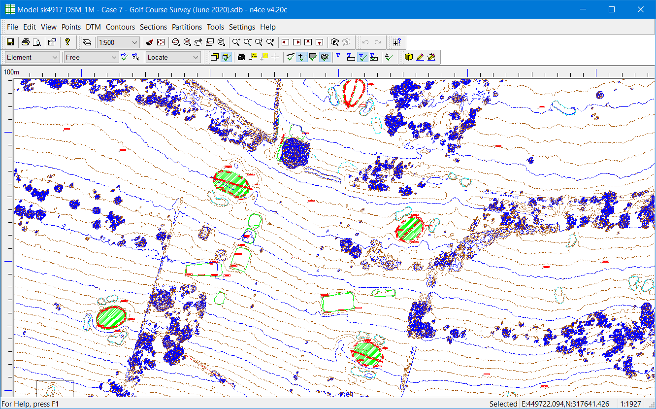
Contours from SK4917_DSM_1m Closely Matching the Ground Survey
We compared levels obtained by GNSS with those found in the LiDAR grid and were pleasantly surprised to get a match to within 5cm, which is more than acceptable for our needs.
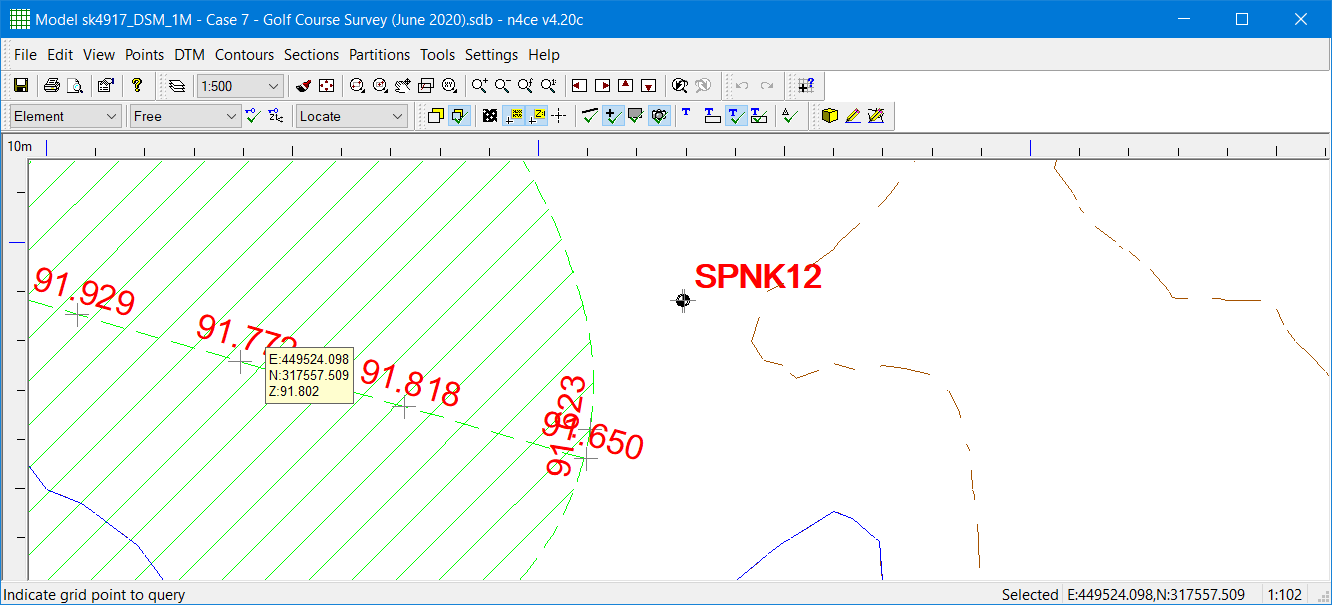
Comparing GNSS Levels with LiDAR Grid Interpolation
We’re now in a position to tidy up our survey, replacing old with updated data. We can then use this updated survey to calculate surface areas of tees, greens and bunkers, digitise outlines of fairways and trees, then finally determine slopes on greens.
The data from the original surveys are held in two model folders called CL 1-18 and Greens, Bunkers & Tees. An updated survey was carried out and stored in March 2017 and the main LiDAR grid file that covers the course is stored in a model called sk4917_DSM_1M.
Finally, the orthorectified georeferenced aerial photography for the site is stored in a file called gm0426B - rev.ecw.
The coded features are given a string number that represents the hole they belong to. For example, BNK3 would be a bunker belonging to hole 3.
We will be using a number of different tools to update the original survey. Clearly, we could simply add the updated survey to the original, but then we’d have two or more overlapping features making it difficult to identify the latest.
One solution is to backcloth the updated survey to the original but in highlight colour. This is exactly what we did here on the 11th green.
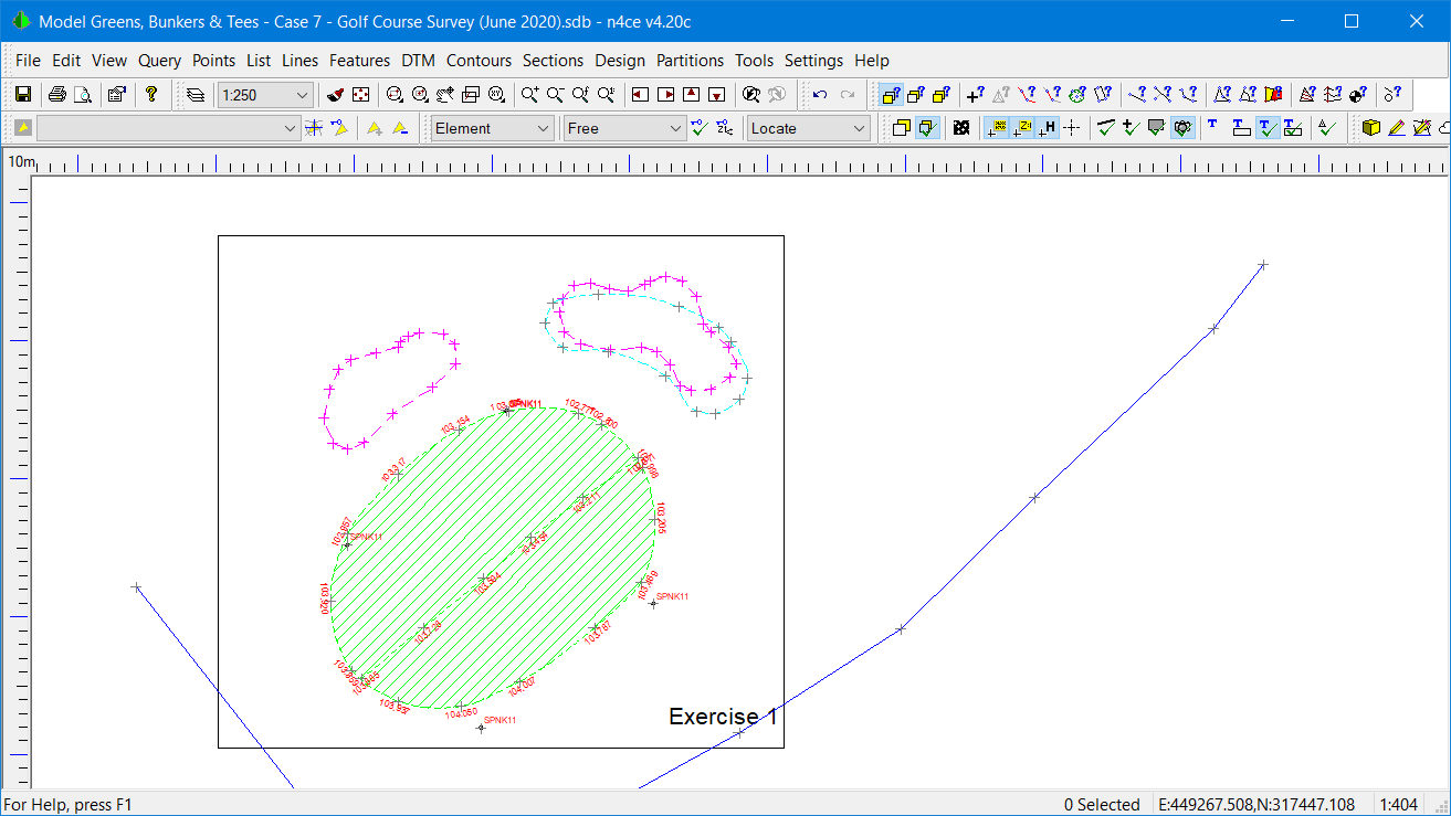
Adding New Bunkers to 11th Green
The original bunker was replaced with two new bunkers, shown in magenta in a backcloth. We can now delete the original bunker outline and copy the two magenta outlines into the foreground original model. And, just to confirm that this is correct we can add the imagery to the backcloth.
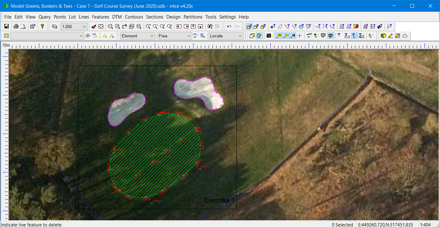
Confirming New Bunker Positions using Imagery
Since we have both registered imagery and LiDAR data, if we missed some detail we can add this by digitising. In the next exercise, we will digitise the outline of a new tee box, removing the old outline.
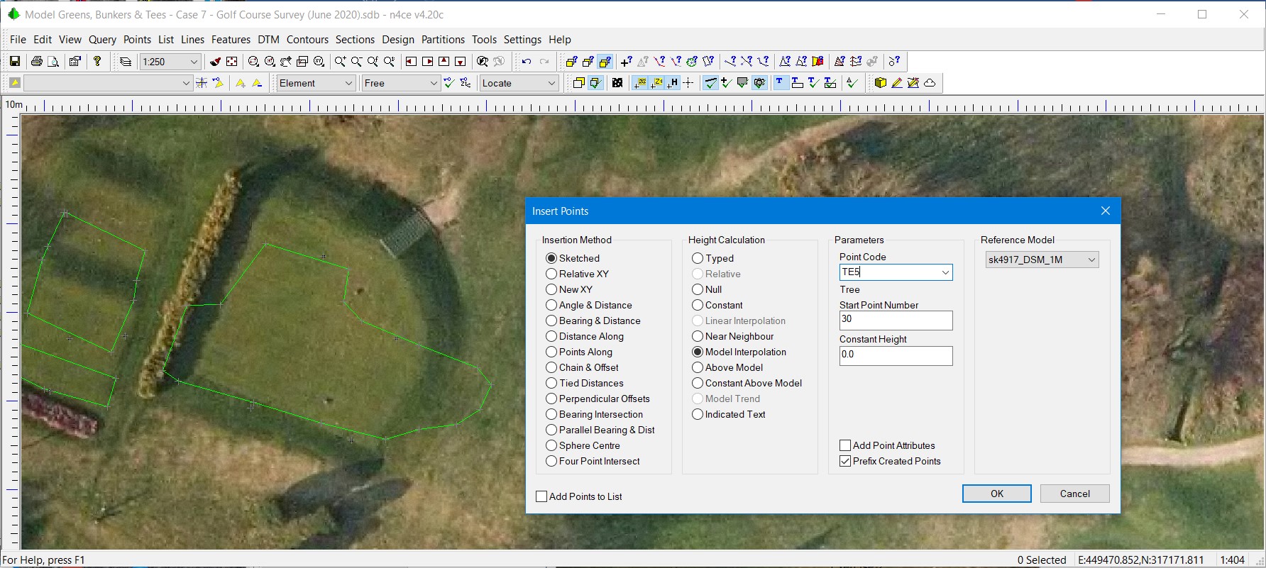
Digitising Revised 5th Tee Box
In this exercise, the old bunker outline can be seen, together with the “new” outline. Use the Points --> Insert option and set the code to TE5, with Model Interpolation using Reference Model sk4917_DSM_1m.
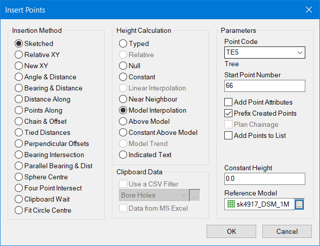
Inserting New Points (updated dialog)
Whilst here we will also add the top and bottoms of the banking. As a check, go into the query string option and see if the string levels are smooth, as expected. Here we can see a spike. This is because there is a tree overhanging the bank, which can clearly be seen from the contours of the LiDAR file. Two options are available to us here. Firstly to remove the offending point or secondly to smooth the string using points on either side of the spike.
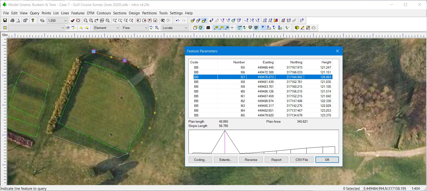
Querying Batter String with a Spike
Clearly, if we are using the LiDAR file to provide levels, we have to make sure spurious levels are not being picked up and if there are sharp changes in slopes or ditches, these should be surveyed directly. The LiDAR file provides a 1m square grid of points and may ignore these features.
The head greenkeeper wanted to know the plan areas of greens and tee boxes. Firstly, make sure each bounding string is complete by joining any breaks and removing overlaps, then use the query string option, as shown above.
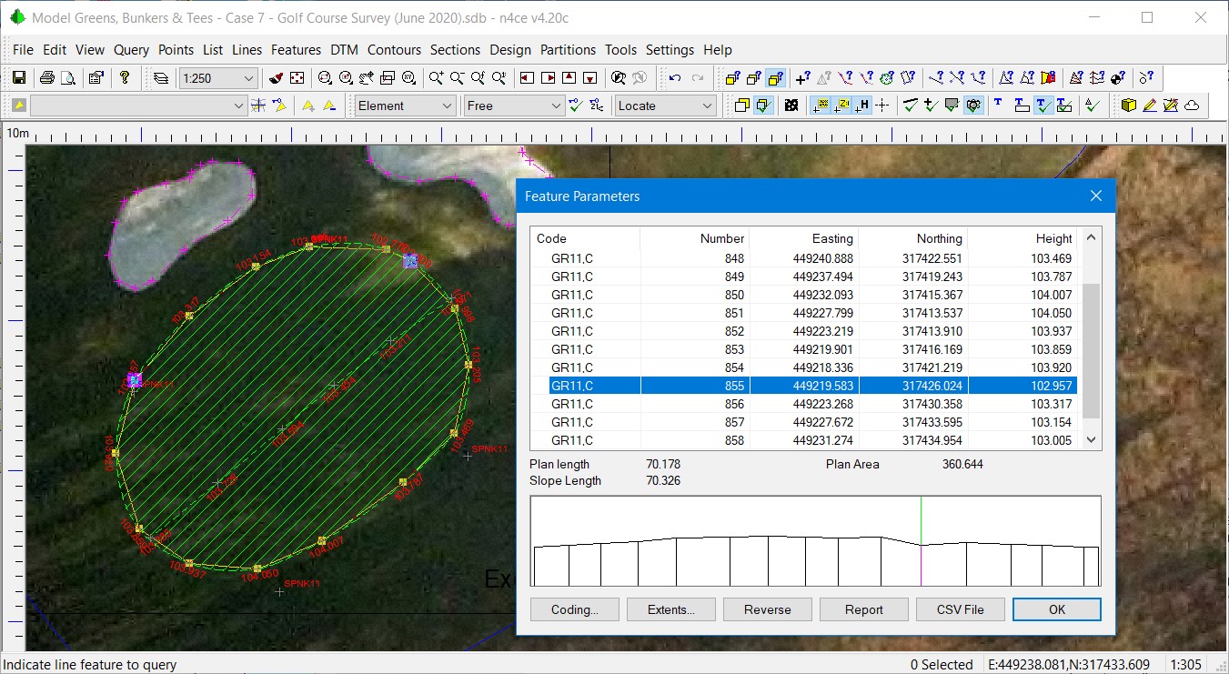
Query String
Note: a vertical profile of the string will be presented. If you highlight a point in the list as above its position will be identified in the profile with a vertical line and in the plan by a purple blob. Double-clicking on the point highlight takes you into the Point Query, allowing you to make changes, for example, its height. This could have been used to correct the height in the above exercise.
Finally, let's see if we can see representative grades on the greens, using the LiDAR data, which we’ve already identified as being accurate to +/- 5cm. In a perfect world, we’d need to carry out a total station survey on each green, for greater accuracy.
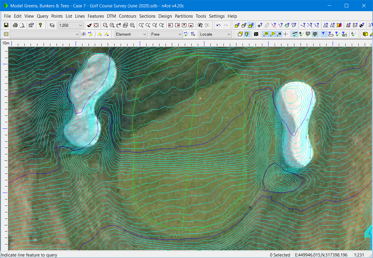
Contour Mapping Greens
In the example here, we’ve set the contour intervals for the LiDAR backcloth to major 1m (blue) and minor 0.05m (cyan). The contours should be smooth, but it does indicate trends that may be useful to golfers. But, remember that the contour maps are justified northerly and not in the direction of the fairway.
Update August 2020
A GNNS survey of the new 5th tee box was carried out and compared to the digitised strings created in one of the exercises above, using the geo-referenced image and LiDAR data. Results showed that both positioning and levels were within tolerance. Here you can see the new steps that were modelled in n4ce and superimposed onto LiDAR and imagery in 3D. A tool is available to automatically generate the steps.

Carrying out GNNS Update Survey on 5th Hole New Tee Box
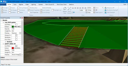
Model Of Update Survey - New 5th Tee Box
Summary Case Study 7
In this case study, we investigated how we could carry out a survey of a golf course, using different data sources. We also looked at how we could edit the survey when changes were made to the course, using the backcloth facility in n4ce.
The next Case Study will also be looking at Longcliffe Golf Course, designing a new teeing area. Much of the data used in this exercise comes from the above with additions using a drone survey.

Comments
0 comments
Please sign in to leave a comment.