
The DTM Advanced option from the Design Menu give you access to some advanced DTM options. When selected, the pop-up menu to the right will be displayed.
Height Factoring
The Height Factor option allows you to factor the heights of a model in relation to another DTM. The factor that is required is expressed as a percentage of the height difference between the current model and the reference model. This factor will only be applied at a point in the current model where a height can be interpolated from the reference model using the same co-ordinates.
If height can be interpolated, the equation used to calculate the new height will be
HNew = HRef + (HOld – HRef) * (1 + k / 100)
where HNew is the new height of the point
HRef is the interpolated height
HOld is the original height of the point
k is the DTM height factor
DTM factoring can be used to predict the settlement of a reinstatement. Once a site has been reinstated, over several years settlement of the deposited material will change the contours. To predict a settlement, the DTM height factor that is required should negative so that if reduces the difference in height between the two models. DTM factoring can also be used to allow for settlement when a reinstatement takes place by increasing the height difference between the models. In this case, the DTM height factor to be applied should be positive.
 |
 |
 |
|
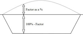
OGL Before Factoring |
Reference Surface |
Resulting Factored Surface |
The three images show the kind of results that can be expected when applying a height factor to a DTM.
Surcharging
The Height Surcharge option allows you to surcharge a DTM by applying a height which will be added to all points in the model You will be asked to enter a change in height to apply. This could be used to simulate a topsoil strip of a site, in which case you should enter a negative change, or the addition of macadam over a carpark, in which case you would enter a positive change.
Addition and Subtraction
The Height Addition and Height Subtraction options allow you to add or subtract a height value that is interpolated from a reference DTM, which would normally represent thicknesses. The information could be used to extrapolate information about geological strata using borehole information.
The example section on the next page shows a ground survey represented by a magenta profile. The other two profiles represent a borehole survey with the blue profile showing the model created by the ground levels of the boreholes and the green profile showing the model created by one of the strata taken from borehole information. In this case, assume it could be the rock head. You can see the problem with this data where the rock head profile is, in places, above the ground which is probably not the case. It is more likely that the rock head will follow the ground profile where no borehole information exists.

To create a more accurate model of the rock head, you should carry out the following steps.
- Create a new model which is an isopachyte model of the difference between the borehole ground level model and the rock head model.
- Create another new model that is a copy of the existing ground model to preserve the original.
- Whilst viewing the copied model, select the Height Subtraction option and, using the resulting dialog box, select the newly created isopachyte model as the reference model to subtract.
Where a point in the existing ground model can interpolate a height from the isopachyte model, this interpolated value will be subtracted from the point’s height. If you create a section through the original ground model and the rock head model resulting from the above operations, you should see section profiles like that below which shows the original ground survey in magenta and the newly calculated rock head surface in blue.

The Height Addition option would add the interpolated heights and can be used in the design of land fill cells.
Care should be taken when using these options as it can only use the data it has to predict the underlying surface and more boreholes would obviously increase the accuracy. However, faults cannot be predicted or handled, and some results will require further attention. In the example above, the little peak in the middle of the profile appears odd and if, after investigation, it turns out to be deposited material, it should probably be removed.
Visibility Calculations
The Calculate Visibility option allows you to carry visibility analysis for one of two possible scenarios. The first is showing what can be seen from a given point and the second is showing where a point is visible from. It is not only a useful tool in supporting planning applications but can also be used to help in the design bunds for landscaping and screening work. When you select this option, the first thing you must do is to indicate the point of interest. This may be the top of a building which you are planning to build. It could also be the front door of somebody’s house where they have objected to a planning proposal. After selecting the point, a property sheet allowing you to set the parameters of the analysis is displayed.

On the Settings page of this sheet, there are two fields called Origin Level and Offset Height and it is important to understand what values you need to enter in these two fields. The Origin Level field will have a default value which is the height of the point that you have indicated.
If you are analysing what you can see from the indicated point, you would normally increase the value in the Origin Level by your height and set the value in the Height Offset field to be 0.0. If you are analysing where the indicated point can be seen from, you may leave the value in the Origin Level as it is and set the value in the Height Offset to be your height. In the situation where you would like to analyse the impact of a new building, you should add the height of the new building to Origin Level field.
The visibility analysis uses radial sections as its basis. Each section is analysed based upon a start height and an observer height to see which parts of the DTM are obscured by its topography. The elements of the sections which are visible or hidden can then be plotted in different colours as radial hatches. You can use the Plot Visible and Plot Hidden check boxes to control which elements to create. Colours and layers are controlled by the settings in the Plot Attributes group. The Show Sections check box allows you to view the sections that are created to carry out the analysis. If they are shown, you have the option to save the sections for later plotting.
The Bearings group defines the directions at which the cut lines radiate out from the point of interest. You can constrain the sector to which cut lines are created using the Start and Finish fields. The cut lines will start at the start bearing and be generated around the point of interest in a clockwise direction until the finish bearing is reached. If you were only interested in the northeast quadrant, the start bearing would be 0° and the finish bearing would be 90°. The Interval field is the angular interval between cut lines. Using the example above, an interval of 10° would generate 10 cut lines. The Full Circle check button allows you to specify that you wish to take sections through 360°. The Distances group defines the length of the cut lines. The values in the Start and Finish fields define the distances from the point of interest of the start and finish of the cut lines.
It is often the case that you are carrying out a visibility analysis of a design model and would like to include a secondary model containing additional data representing the area surrounding the design. This data could come from other sources, such as LIDAR.
The Models page allows you to select this secondary model. You should ensure that the design model remains at the top of the Selected list and move the secondary model across. Any further models will be ignored. When the visibility analysis is carried out, the design model has priority and the secondary model is only used where there is no vertical profile from the design. Effectively, the design model is cut into the secondary model. After you have set all required settings, the sections will be calculated, and the visibility analysis performed. The required hatches representing visible and hidden detail will be created.
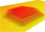
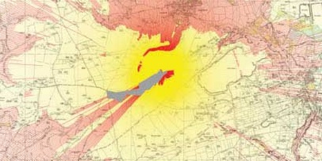
In the example shown above right, it was required that a tall building be built inside a quarry. The quarry is represented by the grey area in the centre of the image. The yellow shaded areas show where the top of the building is hidden from view whilst the red shaded areas shows where the top of the building is visible.
Trend Surfaces
DTM trend surfaces are theoretical planes that stretch off to infinity in each direction. It is normally used where additional points are needed outside the scope of the existing model, such as extending the information for borehole isopachyte models. After a trend surface has been calculated, it can be used to calculate point heights in the options for inserting new points, moving point heights and generating new points from CAD information.

To create a trend surface, you should add the points that you wish to use to the point list. The trend surface is a best-fit inclined plane surface and, therefore, you will need to have selected at least 3 points. You then select the Trend Create option and the equation of the trend surface will be calculated and the surface parameters displayed is a simple dialog box.
The equation of a plane is of the form z = ax + by + c, where a, b and c are constants. In the Trend Surface Parameters dialog box, the value next to Constant represents c, that next to X Coefficient represents a and that next to Y Coefficient represents b.
All the points in the model are then checked against the trend surface and the Height Differences group displays some of the results. The Maximum value is the maximum height difference of a point above the trend surface, the Minimum value is the maximum height difference of a point below the trend surface and the Average value is the average of all the height differences.
The Trend Delete option will delete a trend surface that has been calculated. The Trend Parameters option will display the current trend surface parameters using the dialog box described above.
Comments
0 comments
Please sign in to leave a comment.