Least Squares Network Adjustments

The Least Squares (LSQ) survey engine in n4ce allows multiple control observations between any number of setups to be adjusted such that each individual observation is corrected to arrive at the best fit station coordinates for the unknown setups.

Each observation is split up into its component slope distance, horizontal angle and vertical angle measurements. These are combined with weightings which allow a small degree of movement to be applied to each component. Various equations can then be setup which are solved via large matrix operations.  The stations can be thought of as points hanging in space, in between which are strung springs/observations to tie them together. The larger the weights applied to the springs, the more movement is allowed.  The smaller the weights, the more tension is added to the spring so that it pulls harder.  All of these constraints come together to locate the stations in space. Thereby adjusting weights, will allow the stations more or less freedom to move about. The LSQ process is iterative, so once new locations for the unknown or approximate stations are  determined, the difference between the old and new is examined.  If the differences are outside threshold values, then the process is repeated with the new station locations.  The idea being that the solution will converge to a point that that change is so miniscule that no appreciable change has occurred and the process stops. 

Before using the LSQ adjustment routine at least one station must me known, and a bearing somewhere between stations (that have observations between them). Or, two or more fixed points.  In this case however, the fixed points should be at the extremities of the site, and not to close together. The reason being that fixed points also fix the scale between them, so a short backsight baseline will introduce large scale errors if the overall size of the network is significantly larger.

Starting an adjustment

Right click the survey job folder and select Least Squares to start the process.  After a brief pause the LSQ interface will be displayed.  If there are multiple observations from one setup to another, these will first be averaged.  If any of the spreads of these averages is beyond a predefined tolerance, then a warning message will appear.

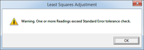
When this occurs the raw readings should first be checked by clicking on the readings tab to see if there is an issue that needs to be resolved. 

Observations with spreads out of tolerance are coloured in red. Hovering the mouse over them reveals the magnitude of the error. The user then needs to decide if the adjustment can continue as a result. Large errors of say many thousands seconds in any angle, or equally large spreads in distance usually point to a station naming error.

Explaining the GUI

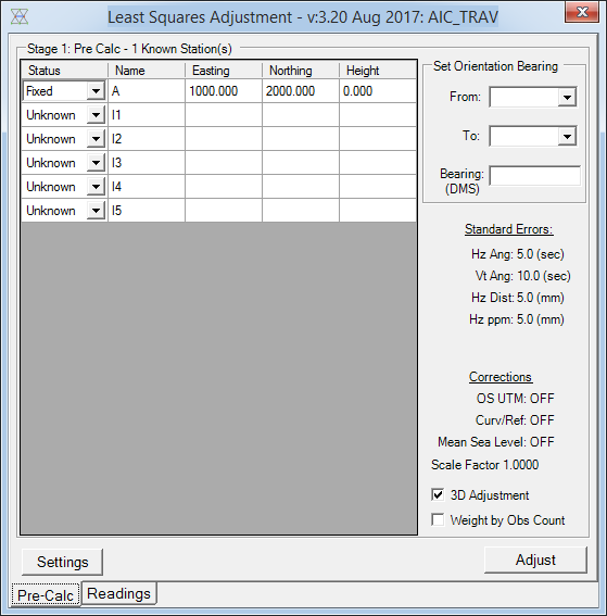
The front end of the LSQ engine lists all of the stations within the project, and what is known about them.  The first stage of the LSQ calculation is to derive approximate coordinates for all stations. Stations that come into the process with Known positions will become Fixed. Fixed points can not move, so should only be input when they are known with a high degree of certainty. If the stations come in as known, but their position is in doubt, then their status should be changed to approximate so that their position can be properly determined. Stations with totally unknown positions will only be included if they can be derived by standard trig or free station calculations before passing them onto the main LSQ algorithm.

Understanding Weights

Key to a successful and accurate adjustment are the weights, these are configured via the Settings button.

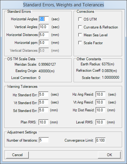
The Standard Errors/Weights are tuned via the boxes provided. These values should be changed based on the accuracy of the survey instrument.  For instance a 5" instrument will probably require a greater degree of movement in the angles than 1".  Typical values for a standard topographic survey are shown above. Usually its a good idea to allow a little more movement in the Va as they need to agree with both target and instrument heights.  Over short distances this can lead to misleading errors being reported as the heights need to be measured very accurately to agree well with the recorded vertical angles.

If the adjustment is using stations with actual OS coordinates, then the OS UTM correction must be enabled. Otherwise the horizontal distances will not be factored down by the appropriate scale factors and the adjustment will result in large errors.  It is down to the user to decide if those distances need to be scaled further by curvature and refraction or mean sea level corrections.  If the site is not in the UK, and the local scale factor is known, then that can be entered into n4ce Corrections defaults before starting the LSQ engine.

Warning tolerances are setup in the middle section. These are both for checking the spreads when starting the LSQ process and also checking for large residuals and RMS errors that are a byproduct of the LSQ operation.

Setting a bearing

Assuming the tolerances are all set accordingly the adjustment can continue if the minimum start conditions have been met. As stated previously this is either one fixed station and a bearing between two stations in the network. Or or two fixed points anywhere in the network, preferably as far apart as possible.  The example below has station A fixed, and is fixing the bearing from A to I5 as 145° 47' 22". 

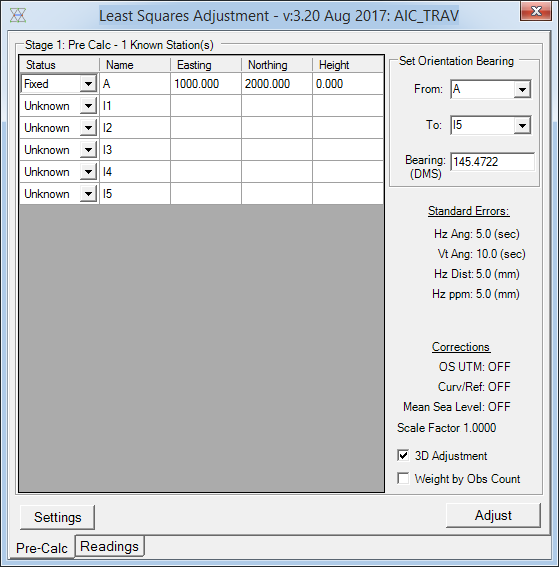
With the conditions set the other considerations are whether or not the adjustment should be 3d or not, and if multiple shots at a setup to the same station should be weighted higher.  i.e. where a leg in a network needs to be strengthened, this weights the observations proportional the number of observations taken to each station. In this situation multiple longer shots benefit more. Especially over shorter ones as shorter readings tend to have greater variation in their spreads. 

Interpreting the results

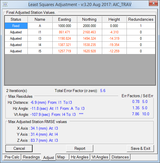
Key to immediately understanding if the LSQ process has resulted in a good overall adjustment is the Total Error Factor, or Sigma Zero value.  The ideal value for this is 1. However, anything between 0.5 and 1.5 is a good target to aim for.

This number can be imagined as a statistical goodness of fit of how well the weights match the quality of the observations.  Very low values signify that more movement is being allowed for than is perhaps necessary. However, that assumes sensible weights.  If something like 60 seconds and 100mm have been input, then it would be no surprise to end up with a small sigma zero value.  But it would mean the overall adjustment was a nonsense. 

If the sigma zero value is in the 0.5 to 1.5 zone, it generally signifies that the weights are in tune with the quality of the observations. Anything less than 0.5 and the weights can probably reduced to not allow as much play as before.

Values significantly over 1.5 can start to indicate the opposite.  i.e. more movement/ larger weights are needed to get everything to agree. This generally points to problem observation(s) somewhere in the network. Again, just resetting and starting everything again with more statistical play in the angles and distances does not a good adjustment make.  The sources of error need to be found and removed before re adjusting with weights that match the accuracy of the total station.

Below the sigma zero value the largest residuals are listed for each component of the adjustment. Along from which are the error factors for each.  These are exactly the same type of error factor as the sigma zero value but this time there is one for each component type.  For instance the value of almost 7mm on Hz distances seems large, but it's error factor is well below 1.  When we examine this observation more closely however, the reading was over 750M.  Hence the error factor being so low.  As given the length of the observation 7mm is actually very good.

What is not so good though is the error factor for the vertical angle component. This value of 7.8 is far outside the realm of acceptability.  This essentially points towards an instrument/target height measurement being incompatible with a vertical angle reading.  Just to see if the adjustment improves if we eliminate the vertical element of the survey it's always a good idea to run the process through in 2d as well.  That will quickly confirm whether or not the positions of the stations are ok in plan, and it's a height/vt angle issue somewhere in the network that is pulling the adjustment out.

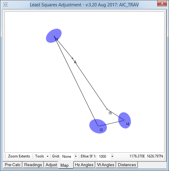
Before making the changes to the adjustment, we should also take note of the Map tab.  This draws the basic structure of the survey, but includes error ellipses (scaled up) about each station.  These are proportional in size to the RMS error of each calculated station, and are orientated in the direction of the largest error/degree of uncertainty. Even though these have been scaled up 1000 times, they should still be much smaller than otherwise depicted.

Returning back to the Pre-Calc tab and unclicking "3d Adjustment" is all that's required to set the process up again to run in plan, and remove any height component.  As there are now approximate coordinates for all of the stations, a message box will appear asking if they should be reused.  As nothing else has changed to effect the location of the survey, we can just press Yes to continue.

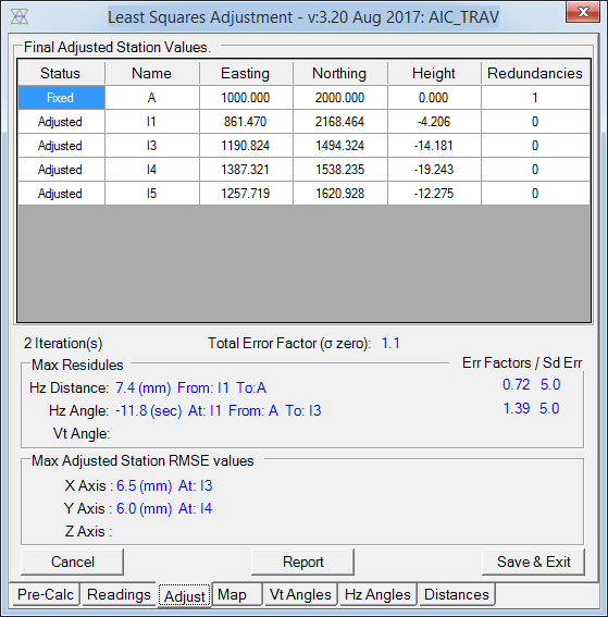
Its immediately apparent that treating this as a 2d problem has eliminated the large errors and brought the sigma zero value down to almost the perfect value. The RMS errors are many times smaller than before and the map view has changed considerably too.

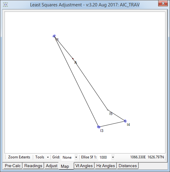
This confirms our original suspicion that either an erroneous vertical angle or height reading of some sort is the reason the original LSQ adjustment has such a large sigma zero value.  What LSQ is able to do however, is identify within the observations the setup at which or two which the issue(s) occurred. To do this the adjustment first needs to be re-run in 3d so we can examine the original results.

Looking at the results it is apparent that all of these residuals occured looking at I3. We have already seen that given the distances involved, the horizontal distance and horizontal angle errors are with tolerance.  Its the vertical angle which is causing the biggest problem.  As such we can deduce that its either a target height or instrument height at or from I3 which is to blame for the excessive vertical angle residuals.  Assuming the vertical angle readings are good, there would need to be a greater degree of movement (larger weight) in the vertical angle in order to get the sigma zero value down to acceptable levels. Obviously this would be very bad practise, so if the 3d element of the survey is required, I3 would probably need to be repeated in order to gain accurate reading that will satisfy the sigma zero tolerance.

Reporting

The map view together with the Vt & Hz Angle, Distance tabs all help to provide greater detail as to what the LSQ adjustment has actually done.  The map view provides a graphic view which can be zoomed and panned so the overall shape and structure of the network can be checked.  Overlaid on to of this are the error ellipses which help track propagation of any errors. The other three tabs list the observations split into their components and document the residuals (correction) assigned to each observation.

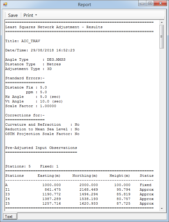
By far the best tool for examining the results is the full report which is accessed via the Report button on the Adjust tab. This report can be printed or saved to disk, but not edited.