LiDAR is a method of surveying which measures height and location detail using pulsed laser light, much like contactless total station distance measurements, or scanning. The acronym comes from Light Detection And Ranging, with data stored in a regular grid format.
For most modelling applications using randomly located data, a triangular DTM will suffice. However, there are increasingly more surveys being created using regular grid data, especially where mass data is involved. Sources of gridded data include UAV’s and scanners, creating point clouds. These contactless surveys generate vast amounts of data, running into tens of millions of points. Tools are available in n4ce to convert point clouds to a LiDAR grid format.
The advantage of this mass gridded data collection is balanced by its accuracy. Clearly, only levels can be recorded at regular intervals, possibly missing interesting detail. There are no features. Secondly, the accuracy LiDAR data is quoted at is +/- 10cm, or sometimes worse.
ASCII XYZ gridded coordinate data can be imported into n4ce using a CSV filter, to generate a triangulated DTM for contours, sections and volumes, but this is a very inefficient way of handling this type of data. n4ce has a facility to import and record gridded data as an array, simply storing the heights at the intersection of nodes. The grid size is used to find the cell of an XY coordinate point. A weighted distance interpolation is then used to find the height of the point in the cell. The sides of each cell can be used to calculate levels along cut lines, when taking sections.
|
The grid cell indices: i = X / Grid j = Y / Grid
Levels: H1 = Height Array (i, j) H2 = Height Array (i + 1, j) H3 = Height Array (i, j + 1) H4 = Height Array (I + 1, j + 1) |
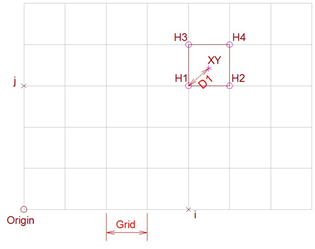 |
Level of point XY = (H1/D1 + H2/D2 + H3/D3 + H4/D4) / (1/D1 + 1/D2 + 1/D3 + 1/D4)
Contours are automatically generated using the cell edges and the diagonal between two corners, according to the current contour default setting, which can of course be changed.
This could generate masses of segmented lines so a levels of detail feature is built in. As you zoom into the grids, more contour lines will be shown. Less will be shown at full zoom.
When importing a grid, it’s possible to attach an image as a backcloth, which also appears in the 3D viewer.
Contour options and layering are the same as triangular models, including layer override (ALT+F9).
In the view shown below, additional modelling options are available which will be discussed later, including editing the grid.
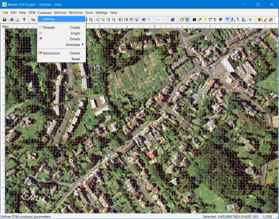
Editing tools are ONLY available in the n4ce Designer edition, but imports and referencing are available in both Lite and Professional editions.
Gridded data can be imported into n4ce in several ways, depending upon content. If the data is in XYZ format then use the From Grid File option.
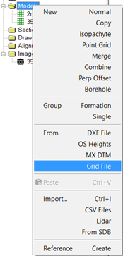
Model Creation – Grid Import
A dialog appears identifying the content of the file. The file extension does not matter here.
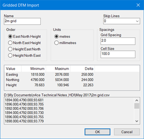
A window at the bottom of the screen will show the contents of the file you are trying to import. You can change the order of coordinates and remove a header.
The alternative data format is already in an array format. In this case, we are looking for files with an ASC or DEM filename extension. The header block to these files contains the number of columns, rows, cell size and bottom left coordinates, as shown below. Use the option Import Lidar in the model creation menu.
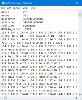
Grid Data Format – Viewed in Notepad
Use the option Import Lidar in the model creation menu. Several options are available here, including the attachment of an image which must be geo-referenced. ECW and MrSid files are the only ones currently supported here.
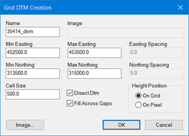
Whilst the size of the grid in this case is 2000m at 2m spacings, it is recommended that you use Disect Dtm into sub-grids for more effective data access. The number of points recommended here is a Cell Size of 500, so 4 individual grids will be created. In situations where internal points may be missing, for example across water, it is possible to interpolate the missing grid heights using the Fill Across Gaps option.
The special option On Pixel Height Position has been added for situations where the height has been attached to a pixel position rather than grid positions, and only works when images are attached. Use On Grid for normal usage.
Once loaded, the LiDAR grid file will appear with its own model grid icon on the project tree, as opposed to the pyramid icon you get for random triangulated data.

The Code Table is not used here, making storage and data access very efficient. You will not see any features, just grid points and contours. These grid models can be used for generating sections and volumes and in design, just like other models which use the code table to draw detail. Overheads are minimised!
In situations where you wish to combine grid files, this is done by importing the files individually then selecting the models you wish to merge from the display window. Right click over the highlighted models and use either the Grid Combine or Grid Unify options.
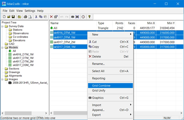
Combining Grid Files
The former option will replace the selected model folders with a single model, whilst the latter will leave the original models in place.
If you have edited the grid model, it’s also possible to export the revisions into a LiDAR file format, so that it can be brought into other packages that support this file format.
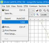
Exporting LiDAR Files
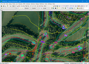
Grid models can be combined visually using backcloths with ground surveys and geo-referenced images, as shown below. Likewise, if they are used in as backcloths they will also be seen in the 3D viewer.
 |
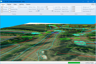 |
| Grid Models Overlaid with Ground Surveys | 3D View of Overlays |
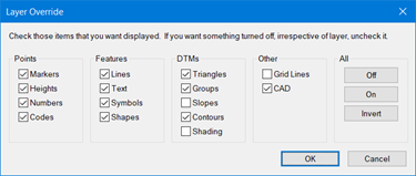
Layer Override
The layer override option (ALT+F9) is supported with some modifications.
Layer Override
The Points and Features options are not implemented here. Only Triangles and Contours are currently implemented in DTMs. The dedicated CAD backcloth is implemented and is where table and curve fitted contours are plotted.
We don’t technically have points in a grid as they are implied where grid lines intersect. If you turn on the tool tip option where the coordinates are shown, the Z value is an interpolated height from the grid and not necessarily at the grid intersection.

If you wish to query a grid intersection, use the Point Query option. Further query options are available in the dedicated CAD backcloth.
![]()
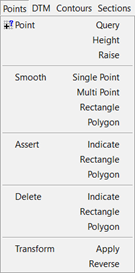
The Point Height option is used to alter the height of a grid intersection (node) by entering a new value. You will be shown the current height. The Raise option will allow you to add/subtract a value from the nodal height.
The Smooth options are used to remove spikes in the model, typically from trees, vehicles or people moving around the site. It helps if you set your contour interval to a small interval to look for spikes, which could also indicate holes.
Several options are available here, including Point and Polygon. In both these cases the heights of nodes in the grid are determined from surrounding points. With Point, you will be requested to identify the node you wish to change first followed by a selection of surrounding nodes that will be used in a weighted distance meaned height calculation for the new node height.
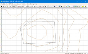
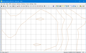
In the case of smoothing by Polygon, a polygon outline needs to be swept out, identifying the nodes inside the polygon that need to be smoothed. The height of nodes directly outdide the polygon will be recorded and used in the calculation of a best fit polynomial surface. Nodes inside this polygon will then be projected onto this surface to determine their new heights.
 |
 |
|
Polygon Smoothing |
|
The Assert options are used to fill in holes, left in the grid and are useful when stitching adjacent grids together, as there is normally a gap. Options include Indicate, Rectangle and Polygon.
The Delete options allow you to remove grid points from the model by Indicate, Rectangle or Polygon. This would normally be applied to grid points around the edges of the model to form a band of interest but see Crop below. Points that have been removed are made into 2D points, leaving holes in the model.
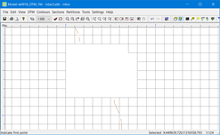
Deleting points in the Grid Model
The Transform option allows uses to rescale about a nominated origin. This can be used if the grid file is in mm, or reversing to change from m to mm before exporting. You will be provided with a Grid transformation dialog, as shown below. A Reverse option is provided as this action is not included in the undo engine.

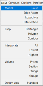
DTM Menu
Several different options are available here, including further nodal height edits, like the Raise option which allows you to alter all the node heights in the grid by a fixed amount. Contours will automatically update to the new grid nodal values.
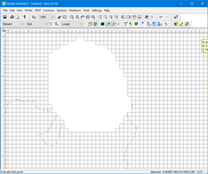
The Edge Assert option is used to fill any holes in the current grid. It uses all the available models in the project, to fill in the gaps.
 |
 |
|
| A Grid with Holes | Post Edge Correction | DTM Menu |
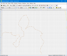
The Isopachyte option creates a height difference model, to a nominated model which must be another grid model. In this case the current model is converted into the height different model, losing its original levels. Isopachytes can be created between two different models and stored independently, using the New option when right clicking over Models in the Project Tree.
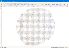
Isopachyte Height Difference Model
The Intersection option works much like a normal triangular DTM and shows where the cut/fill balance is, between two models. You will be invited to compare the current grid with another model which could be a grid or a triangular model. If an intersection is found you will be invited to enter a Coordinate folder name, where the intersection (zero isopachyte) will be stored.
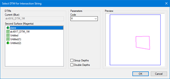
Intersection Model Comparison
The Crop option allows you to remove points outside of a defined boundary, which must be sketched out.
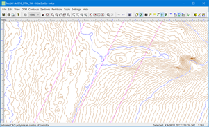 |
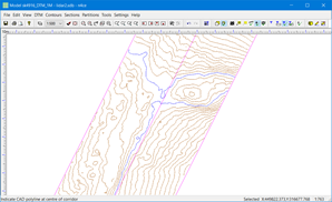 |
Corridor Cropping of Grids
This option should be used to identify the areas of the grid model you wish to keep and is ideal for pipelines and roads design. Points outside of the swept-out Rectangle, Polygon or Corridor will be removed. In the case of a corridor you need a polyline in a separate CAD data folder and use this as a backcloth. An offset from this centerline will be requested.
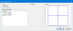
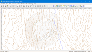
The Interpolate option allows you to blend in another model into the current grid and is particularly useful if you are wanting to upgrade the accuracy of the grid model. Typically, here you would be interpolating to a ground survey model. You will be invited to select the model you wish to interpolate to. It it’s a ground survey it must contain a DTM and is equivalent to the merge option in the normal triangular DTMs. The difference here is that you have the option to update All or purely levels above (Highest) or below (Lowest) on a selection of reference models.
 |
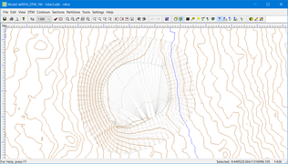 |
Interpolate Models – Before and After
Calculating Volumes
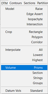
If you’ve made yourself familiar with triangular DTMs, taking sections and calculating volumes, you’ll be familiar with the process here. But there is one proviso!
When calculating volume using triangular DTMs, to projected surface, n4ce calculates a complex surface called an isopachyte model. Where triangles sides from one surface intersection the triangle sides from the reference, new points are identified, with a height difference calculated between the two DTMs.
These new points are included with a double point projection to create a new model called an isopachyte, which only includes the overlapping triangles and honours break lines from both models. The isopachyte is used during prismoidal volume calculations and then deleted. Section volumes use enclose areas between models and hence do not use isopachytes. Group volumes are not available with grids and should be calculated from the regular triangular model, if required.
There is an extra prismoidal volumes option with grids called Simple Projections. When using this option only the height differences at the nodes of the current model projected to the reference surface will be used to create the “toblerones” used in prismoidal calculations. Where there is no overlap the height difference will be assumed to be zero. This method of calculating volumes is very quick but of course is not as accurate as the isopachyte method, but is still useful. When calculating volumes from a grid model to another reference only the simple option is available, but when calculating from a triangular to a grid the isopachyte method can be selected.
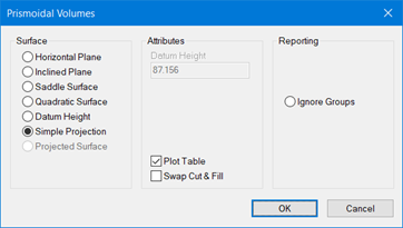
Prismoidal Volumes using Simple Projections (Grids)
|
Note Remember that groups can only be used with triangular models and to switch volumes quantities if you have the final design (triangular model with groups) as the current model and the reference is the original as a grid or triangles. |
The Volume Strings option allows you to calculate the volume of grids identified inside a polygon feature. The reference surface used in these calculations is the model created by the string itself.
Firstly, the model containing the string needs to be identified as a backcloth to the grid model, as shown in the example below. Nodes on the selected string will be highlighted. Since multiple string volumes can be calculated simultaneously, you will be invited to select further strings. Right click to terminate selection.
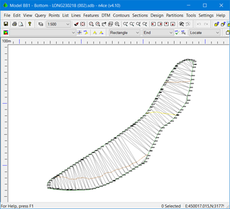
There are several stages to these calculations. Firstly, the grid nodes within each string will be identified and used to generate a DTM. Secondly, the string will be used to calculate a reference surface (DTM) and finally the isolated grid points will be projected to the string DTM to calculate an isopachyte which is used to determine the volume between the grid and the reference string models.
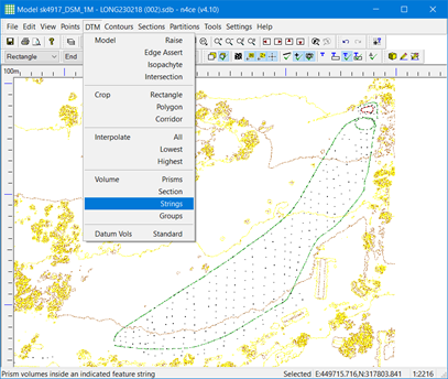
 |
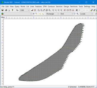 |
String DTM Grid DTM
You will be given the option to save these two models, as shown above, but this is not fully necessary as they will be formed then deleted after the calculation process.
The Volume Groups work very similar to the volume from strings except you will be working with groups stored in a triangular DTM backcloth. In this instance the grid becomes the reference surface****? To be completed!!!!!
Finally, the Datum Vols Standard is used to calculate quantities from a reference datum, that you supply. There are several options here, as is shown below.
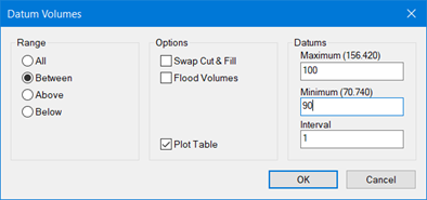
Datum Volumes Options
The results provide you with incremental quantities of volumes above and below datum values between incremental changes.
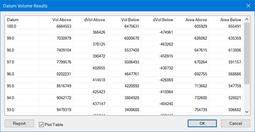
Report for Volumes Between 90 and 100 in Increments of 1m
The Flood Volumes option allows you to ********************. To be completed!
The example we use below, is of a reservoir and the exercise is to calculate volumes of material and void as its filled in increments of 0.5m. You will be shown a Report and given the opportunity to plot a Table.
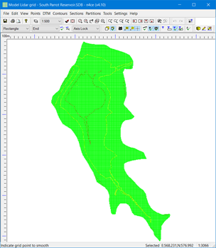
LiDAR file of a Reservoir
Note there is another option when using normal triangular DTM’s that allows you to “fill” the cavity, plotting hatch to show the outline of the fill. This is called Contour Volumes but is not available with LiDAR grids.
Contours
The contours menu work very similar to the Triangular DTM, in that contours are displayed automatically based on the current Settings. Once you have loaded your LiDAR grid contours will appear and redraw as you zoom in and out, the only difference being we use levels of detail here. This means it only show you outline contours. As you zoom in closer, more contours will appear, this speeding up re-draws. After editing the grid contours will update automatically.
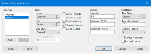
Contour Settings
Since these contours, like the triangular model contours, are drawn on the fly, exporting these to a DXF/DWG file would generate lots of individual line segments. We would recommend that you generate threaded contours first.
Each grid model has a dedicated CAD backcloth, just like triangular models, which is where tables and threaded contours are stored. Use the Threads Create, Single and Annotate to generate and annotate these CAD contours. But remember that these contours will not update if you do further model editing.
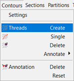
Grid Contours Menu
Taking Sections
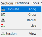
Grid Sections Menu
Menu options are available for generating sections directly from the grid model, but the grid can be referenced elsewhere in the project for both sections and volumes. Levels from the cut line will be interpolated along the side of each grid they cut and a diagonal between opposite corners. Viewing, saving and plotting is the same as triangular models.
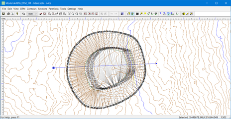

Taking and Viewing Sections
Remember, grid models have the same overall structure as normal model and support both the dedicated CAD backcloth and layer overrides [ALT+F9].
The Contours, Sections, Partitions and Tools menu options are not fully discussed here as they are self-explanatory, if you are familiar with the same tools in a triangular model.
|
Please be aware of the prompts, seen at the bottom of the screen, when you make a menu selection. They will direct you to take the appropriate actions. |
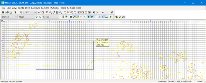
In the example above, we are cropping part of the grid by rectangle.

Comments
0 comments
Please sign in to leave a comment.